


Syntax
=QUERY(data, "query", [headers])
It takes 3 arguments:
Select the data you want to analyze
Query the data
Optional: Number indicates how many header rows there are in your data
Example QUERY function:
=QUERY(A1:D234,"SELECT B, D",1)
The query statement is the string inside the quotes, in green. In this case, it tells the function to select columns B and D from the data.
The third argument is the number 1, which tells the function that the original data had a single header row.
Notes
The keywords are not case sensitive, so you can write “SELECT” or “select” and both work.
If you use column letters they must be uppercase: A, B, C, etc.
Keywords must appear in this order:
select
where
group by
order by
limit
label
Examples
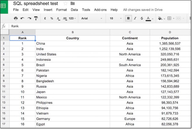
In this tutorial, I have used a named range to identify the data, which makes it much easier and cleaner to use in the QUERY function. Feel free to use the named range “countries” too, which already exists in the template.
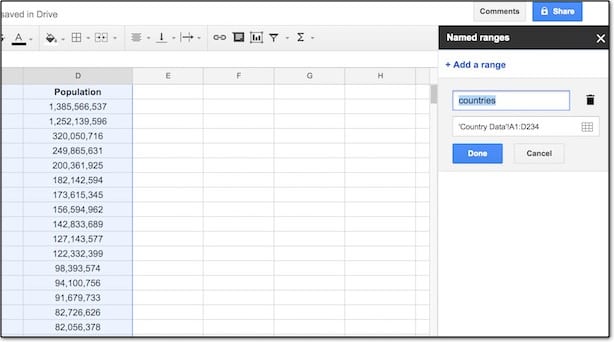
If you’re new to named ranges, here’s how you create them:
Select your data range and go to the menu:
Data > Named ranges…
A new pane will show on the right side of your spreadsheet. In the first input box, enter a name for your table of data so you can refer to it easily.
SELECT All
The statement SELECT * retrieves all of the columns from our data table.
To the right side of the table (I’ve used cell G1) type the following Google Sheets QUERY function using the named range notation:
=QUERY(countries,"SELECT *",1)
Note: If you don’t have a named ranges then your QUERY formula will look like this.
=QUERY(A1:D234,"SELECT *",1)
For the remainder of this article, I’ve used the named range “countries” but feel free to continue using the regular range reference A1:D234 in its place.
The output from this query is our full table again, because SELECT * retrieves all of the columns from the countries table:
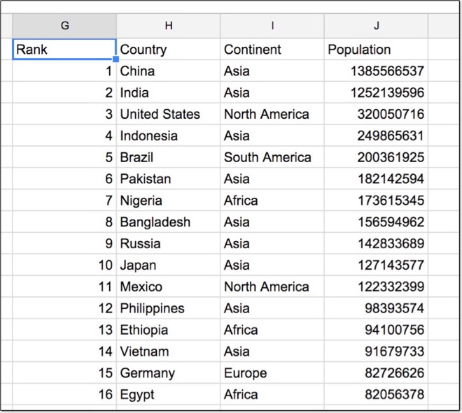
Wow, there you go! You’ve written your first QUERY! Pat yourself on the back.
SELECT Specific Columns
What if we don’t want to select every column, but only certain ones?
Modify your Google Sheets QUERY function to read:
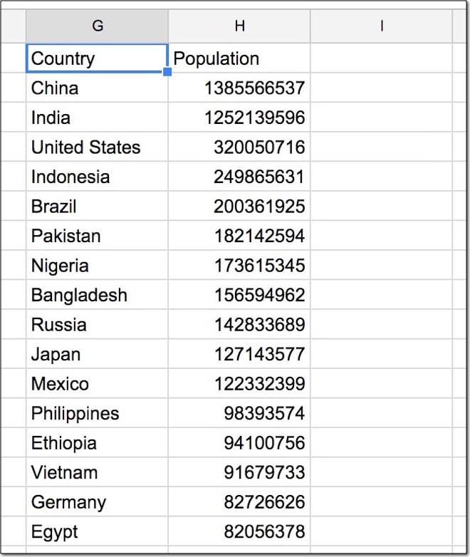
=QUERY(countries,"SELECT B, D",1)
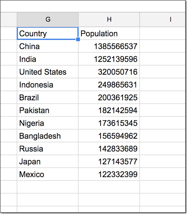
This time we’ve selected only columns B and D from the original dataset, so our output will look like this:
WHERE Keyword
The WHERE keyword specifies a condition that must be satisfied. It filters our data. It comes after the SELECT keyword.
Modify your Google Sheets QUERY function to select only countries that have a population greater than 100 million:
=QUERY(countries,"SELECT B, D WHERE D > 100000000",1)
Our output table is:
Let’s see another WHERE keyword example, this time selecting only European countries. Modify your formula to:
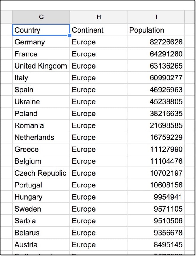
=QUERY(countries,"SELECT B, C, D WHERE C = 'Europe' ",1)
Notice how there are single quotes around the word ‘Europe’. Contrast this to the numeric example before which did not require single quotes around the number.
Now the output table is:
ORDER BY Keyword
The ORDER BY keyword sorts our data. We can specify the column(s) and direction (ascending or descending). It comes after the SELECT and WHERE keywords.
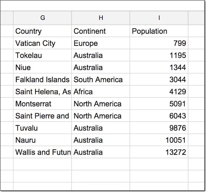
Let’s sort our data by population from smallest to largest. Modify your formula to add the following ORDER BY keyword, specifying an ascending direction with ASC:
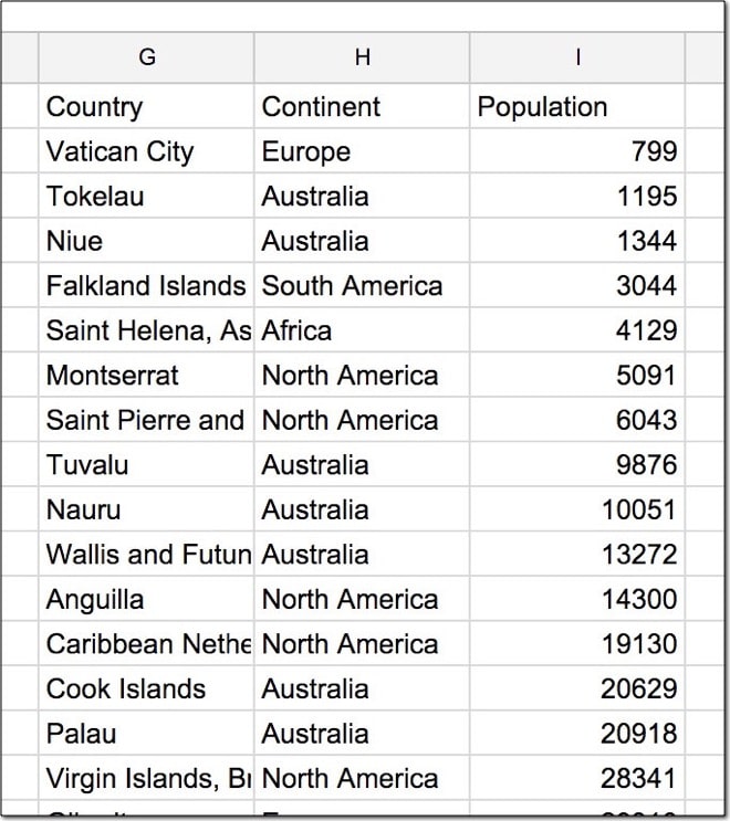
=QUERY(countries,"SELECT B, C, D ORDER BY D ASC",1)
The output table:
Modify your QUERY formula to sort the data by country in descending order, Z – A:
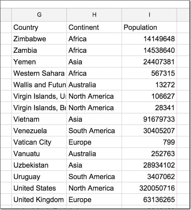
=QUERY(countries,"SELECT B, C, D ORDER BY B DESC",1)
Output:
LIMIT Keyword
The LIMIT keyword restricts the number of results returned. It comes after the SELECT, WHERE, and ORDER BY keywords.
Let’s add a LIMIT keyword to our formula and return only 10 results:
=QUERY(countries,"SELECT B, C, D ORDER BY D ASC LIMIT 10",1)
This now returns only 10 results from our data:
Arithmetic Functions
We can perform standard math operations on numeric columns.
So let’s figure out what percentage of the total world population (7.16 billion) each country accounts for.
We’re going to divide the population column by the total (7,162,119,434) and multiply by 100 to calculate percentages. So, modify our formula to read:
=QUERY(countries,"SELECT B, C, (D / 7162119434) * 100",1)
I’ve divided the values in column D by the total population (inside the parentheses), then multiplied by 100 to get a percentage.
Output:
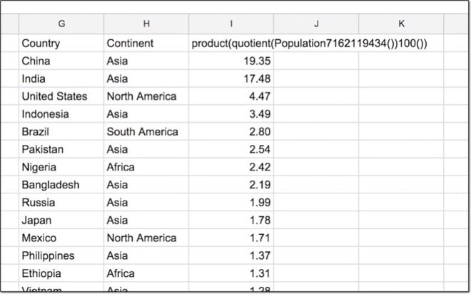
Note – I’ve applied formatting to the output column in Google Sheets to only show 2 decimal places.
LABEL Keyword
That heading for the arithmetic column is pretty ugly right? Well, we can rename it using the LABEL keyword, which comes at the end of the QUERY statement. Try this out:
=QUERY(countries,"SELECT B, C, (D / 7162119434) * 100 LABEL (D / 7162119434) * 100 'Percentage'",1)

=QUERY(countries,"SELECT B, C, (D / 7162119434) * 100 LABEL (D / 7162119434) * 100 'Percentage' ",1)
Aggregation Functions
We can use other functions in our calculations, for example, min, max, and average.
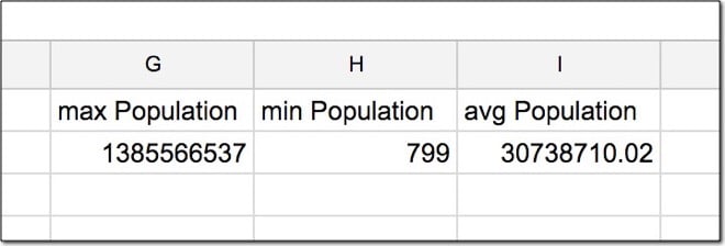
To calculate the min, max and average populations in your country dataset, use aggregate functions in your query as follows:
=QUERY(countries,"SELECT max(D), min(D), avg(D)",1)
The output returns three values – the max, min and average populations of the dataset, as follows:
GROUP BY Keyword
Ok, take a deep breath. This is the most challenging concept to understand. However, if you’ve ever used pivot tables in Google Sheets (or Excel) then you should be fine with this.
The GROUP BY keyword is used with aggregate functions to summarize data into groups as a pivot table does.
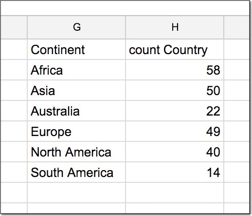
Let’s summarize by continent and count out how many countries per continent. Change your query formula to include a GROUP BY keyword and use the COUNT aggregate function to count how many countries, as follows:
=QUERY(countries,"SELECT C, count(B) GROUP BY C",1)
Note, every column in the SELECT statement (i.e. before the GROUP BY) must either be aggregated (e.g. counted, min, max) or appear after the GROUP BY keyword (e.g. column C in this case).
Output:
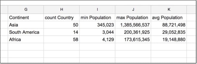
Let’s see a more complex example, incorporating many different types of keyword. Modify the formula to read:
=QUERY(countries,"SELECT C, count(B), min(D), max(D), avg(D) GROUP BY C ORDER BY avg(D) DESC LIMIT 3",1)
This may be easier to read broken out onto multiple lines:
=QUERY(
    countries, "SELECT C, count(B), min(D), max(D), avg(D)
    GROUP BY C
    ORDER BY avg(D) DESC
    LIMIT 3",1)
This summarizes our data for each continent, sorts by highest to the lowest average population, and finally limits the results to just the top 3.
Output:
Advanced Google Sheets QUERY Function Techniques
In addition, there are more data manipulation functions available than we’ve discussed above. For example, there are a range of scalar functions for working with dates.
Suppose you have a column of dates in column A of your dataset, and you want to summarize your data by year. You can roll it up by using the YEAR scalar function:
=QUERY(data,"select YEAR(A), COUNT(A) group by YEAR(A)",1)
Resources
Official Google documentation for the QUERY() function.
Official documentation for Google’s Visualization API Query Language.
https://www.benlcollins.com/spreadsheets/google-sheets-query-sql/